FM with IQ Demodulation

[ radio fm math demodulation ]

After some time reading about hacking RF signals:

• Using RTL-SDR to automatically receive weather satellite images. 
• Reverse engineering traffic lights with software defined radio.
• Spectrum painting on 2.4 GHz.
• RTL-SDR Tutorial: Cheap ADS-B aircraft radar

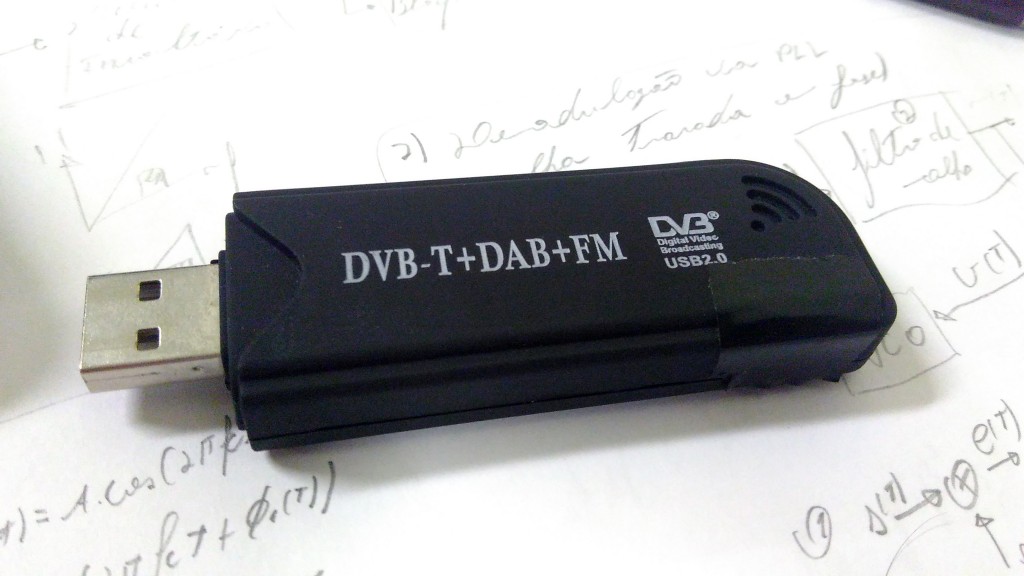
I bought a RTL2832U receiver, that can operate on a range of 70-1700 Mhz.

Aliexpress link.

Libraries and Programs

After some time (6 months, hell yeah Brazil...) to receive the package, I begun to install all the programs and libraries to use the RTL.

$ sudo apt-get install gnuradio rtl-sdr gqrx-sdr

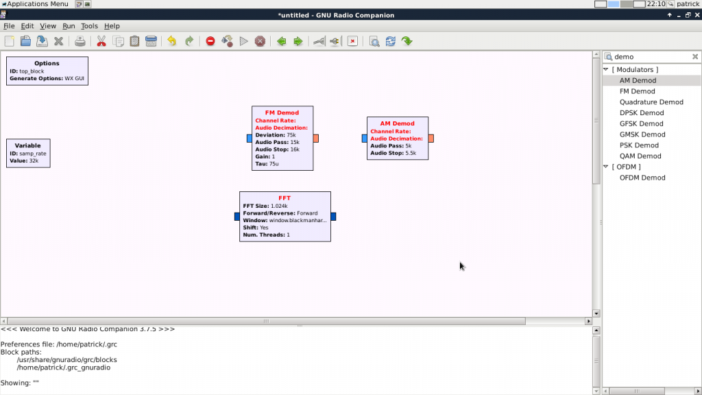
• gnuradio : GNU Radio is a free software development toolkit that provides signal processing blocks to implement software-defined radios and signal processing systems. It can be used with external RF hardware to create software-defined radios, or without hardware in a simulation-like environment. It is widely used in hobbyist, academic, and commercial environments to support both wireless communications research and real-world radio systems. (ty wikipedia).

  

• rtl-sdr have:

`

 * rtl_adsb: a simple ADS-B decoder for RTL2832 based DVB-T receivers
 * rtl_eeprom: an EEPROM programming tool for RTL2832 based DVB-T receivers
 * rtl_fm: a narrow band FM demodulator for RTL2832 based DVB-T receivers
 * rtl_sdr: an I/Q recorder for RTL2832 based DVB-T receivers
 * rtl_tcp: an I/Q spectrum server for RTL2832 based DVB-T receivers
 * rtl_test: a benchmark tool for RTL2832 based DVB-T receivers

`

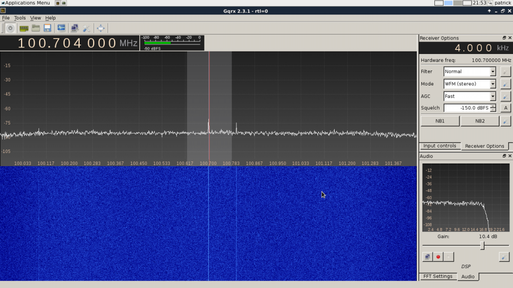
• gqrx-sdr is a RF receive interface that have a displays FFT plot and spectrum waterfall very helpful to detect signals,  the software includes AM, SSB, FM-N, FM-W (mono and stereo) demodulators and Special FM mode for NOAA APT.

After installed all the software and plugging the receiver on the computer, we can see that have a Realtek chip with the lsusb feedback.

Bus 001 Device 004: ID 0bda:2838 Realtek Semiconductor Corp. RTL2838 DVB-T

Ok, now with everything done,  we can capture some data ! We can use the rtl-sdr toolkit.

rtl_sdr capture.bin -s 1.8e6 -f 100.9e6

The capture.bin is the file that will have the IQ data, 1.8 MHz is the sample frequency and the frequency that we will look for is 100.9MHz (Rádio Atlântida), the radio station.

Warning !! 1.8e6 samples for second, so take 3~10 seconds because the fast growing of the file.

To demodulate we need do understand the modulation.

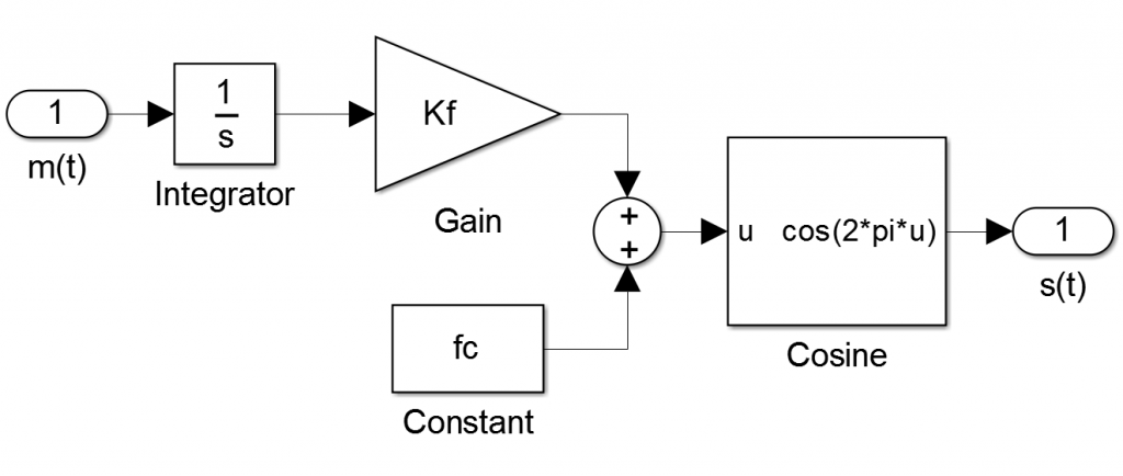
The FM is a method to modulate a message $m(t)$ with the change of the carrier $cos(2\pi f_c t)$ phase's $\phi(t)$. Wikipedia is your friend.

The phase have a relationship with the message, that is $\phi(t) = 2\pi K_f \int^t_0 m(u)du$. So the simple FM modulator will look like:

The $s(t)$ data will be transmitted after the modulation.

Demodulate FM, IQ Decomposition.

The RTL driver give to us the result of the QAM demodulator.

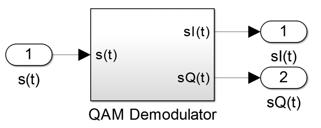Where:

$s(t) = Acos(2\pi f_ct+\phi(t))$ $cos(a+b)=cos(a)cos(b)-sin(a)*sin(b)$ $s(t) = Acos(\phi(t))cos(2\pi f_ct) - Asin(\phi(t))sin(2\pi f_ct)$ $s_I(t) = Acos(\phi(t))$ $s_Q(t) = Asin(\phi(t))$ $\phi(t) = \sphericalangle (s_I(t)+js_Q(y))$

You can read more about IQ data $s_I(t) s_Q(t)$ here.

Now we know how to demodulate the FM, with the equations above, the result is: $m(t) = \frac{1}{(2\pi K_f)} \frac{d}{dt}(\sphericalangle (s_I(t)+js_Q(y))$

Some code.

Now, with the knowledge of how the FM modulation and demodulation work, we can write a octave code that can show to us how the theory work in the real world.

%read file and convert data
fid = fopen('./capture2.bin','rb');
y = fread(fid,'uint8=>double');
y = y-127;
% transform IQ data to an imaginary number
yi = y(1:2:end)+i*y(2:2:end);

% the radio frequency and the sample frequency
freq = 100.9e6;
fs = 1.8e6;

% some math
yang = angle(yi);     % take the angle -pi to pi
yrap = unwrap(yang);  % make the correction to continue the angle after pi and -pi
tdev = diff(yrap);    % the derivative of theta
sound(tdev,fs)        % give us some music

You can download the capture.bin that I have used and the .m code to octave (open source rules) here: fm_demodulator_mono.

Stereo demodulation.

Ok, we have done the simpliest demodulation possible, without filters and a lot of things, so now we will use more energy to obtain a very good  good cool sound.

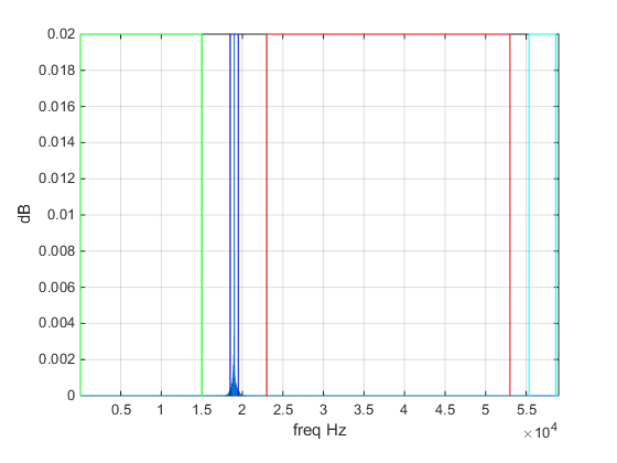
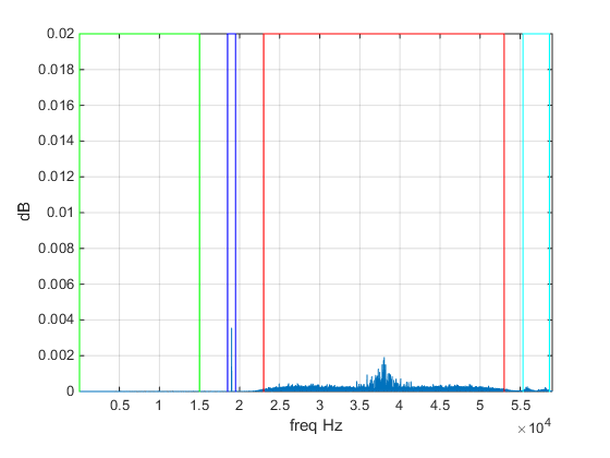
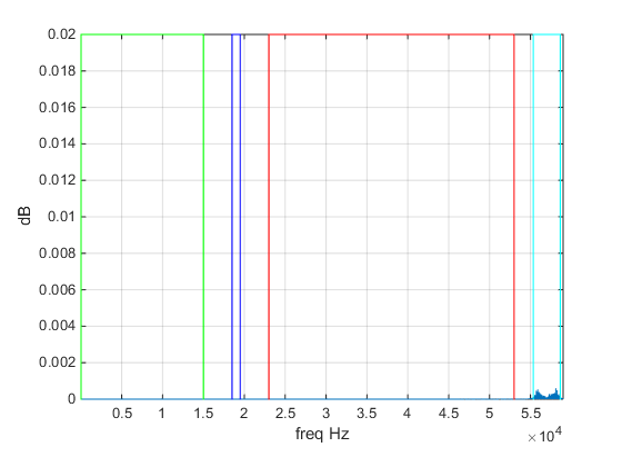
The FM spectrum

The FM spectrum have more things that I thought.

1. 30~15kHz L+R (mono), that we have already demodulated.
2. 19kHz, the omnipotent carrier.
3. 23~53kHz, a kind of dsb-sc (double side band suppressed-carrier) with L-R.
4. 55.35~58.65kHz, the RBDS (Rebeldes Radio Data system),  a kind of digital data system.
5. 58.65~76.65kHz, FTF first read this, now ask yourself wth Microsoft is here ??
6. 92+$\Delta f_{as}$, IDKWII.

What is important ?

The FM modulation appears to be something like this:

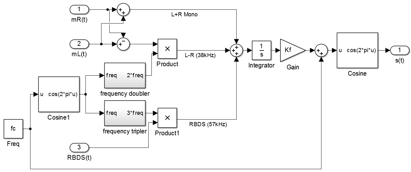
Mathematically:

$s(t) = cos(2\pi f_c+\phi(t))$ Where $\phi(t) = 2 \pi K_f\int[m_R(t)+m_L(t)+ (m_R(t)-m_L(t))cos(4\pi f_c t)+RBDS(t)cos(6\pi f_c t)]$.

Yeah, this is a kind of crazy. The IQ data give to us the imaginary part that compose the $\phi(t)$, theoretically making the FFT of $\frac{d}{dt}\phi(t)$ we can see something like the FM spectrum image.

% fft
 tdfft = fft(tdev);
 P2=abs(tdfft/ysize);
 P1=P2(1:ysize/2+1);
 P1(2:end-1)=2*P1(2:end-1);
 f=fs*(0:(ysize/2))/ysize;
 % plot the fft until 59kHz
 freqe=round(2*59e3*size(f)/fs);
 freqe=freqe(2);
 plot(f(1:freqe),(P1(1:freqe)))
 grid on
 xlabel 'freq Hz',ylabel 'dB'
 hold on
 axis([30 59e3 0 0.02])

 Gab1 = [30 0; 30 0.02; 15e3 0.02; 15e3 0]; % R+L
 plot(Gab1(:,1),Gab1(:,2),'g');

 Gab1 = [18.5e3 0; 18.5e3 0.02; 19.5e3 0.02; 19.5e3 0]; % carrier
 plot(Gab1(:,1),Gab1(:,2),'b');

 Gab1 = [23e3 0; 23e3 0.02; 53e3 0.02; 53e3 0]; % R-L
 plot(Gab1(:,1),Gab1(:,2),'r');

 Gab1 = [55.35e3 0; 55.35e3 0.02; 58.65e3 0.02; 58.65e3 0]; % RBDS
 plot(Gab1(:,1),Gab1(:,2),'c');

And the result:

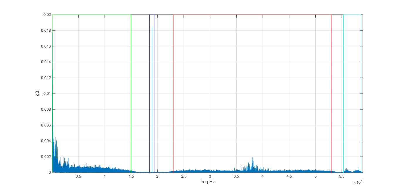
All good, all good sir !

The carrier and his friends.

Like said before, we have the IQ data that can give to us the $\phi(t)$ and with a derivative we can have $m_R(t)+m_L(t)+ (m_R(t)-m_L(t))cos(4\pi f_c t)+RBDS(t)cos(6\pi f_c t)$. Applying a low-pass filter on the L+R, a band-pass filter on the carrier, L-R and RBDS we can have a clear signal of each data.

With the frequencies specifications, the filter was done:

%R+L
[b,a] = butter(10,2*16e3/fs,'low');
R_p_L = filter(b,a,tdev);
hhhh=R_p_L;
plote

%carrier
[b,a] = butter(4,[2*18.5e3,2*19.5e3]/fs,'bandpass');
carrier = filter(b,a,tdev);
hhhh=carrier;
plote

% R-L
[b,a] = butter(4,[2*23e3,2*53e3]/fs,'bandpass');
R_l_L = filter(b,a,tdev);
hhhh=R_l_L;
plote

%RBDS
[b,a] = butter(4,[2*55.35e3,2*58.65e3]/fs,'bandpass');
rbds = filter(b,a,tdev);
hhhh=rbds;
plote

The 'plote' code plot the fft of the signal.

$m_R(t)+m_L(t)$

$cos(2\pi f_c t)$

$(m_R(t)-m_L(t))cos(4\pi f_c t)$

$RBDS(t)cos(6\pi f_c t)$

To be continue..